Home

All SEB tutorials

Tutorial: Semi-flexible polymers with SEB

Contributors: Carsten Svaneborg and Lau Blom Grøndahl (FKF SDU).

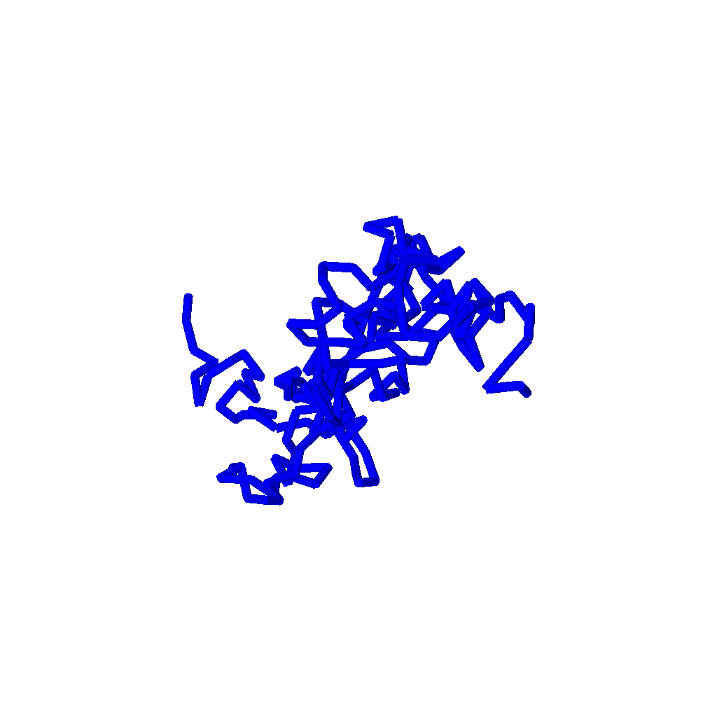
Illustration of a semi-flexible polymer molecule as a chain of rods.

Before you start

• Download and install SEB
• Complete the polymer tutorial to understand the scattering from Gaussian polymers. Here you also learn how to run SEB and use it for calculating scattering profiles.
• Complete the rod tutorial to understand the scattering from thin stiff rods. Here you also learn how to use rods in SEB.
• Complete the chain of rods tutorial to understand how to derive the form factor for a chain of rods. Here you also learn how to connect sub-units together to build structures, and how to use SEB to calculate the form factor of such structures.

Learning outcomes

• comparing a semi-flexible polymer model to a completely flexible Gaussian chain model.

Semi-flexible polymers

In the polymer tutorial, we looked at Gaussian polymer models. That is we regard a polymer as a random walk fractals on all length scales. These models accurately describe the large spatial scale / low $q$ behaviour of polymers, but fail at molecular scales where the molecule is locally rod-like. Rod tutorial we derived the scattering from a solution of rods, and in the Random walk chain of rods tutorial we derived theory for the scattering from a chain of units.

Here we want compare the scattering from a random walk model of a chain of rods to the Gaussian polymer model. We will also compare these scattering curves to scattering curves from polymer simulations.

Scattering Equation Builder (SEB)

Scattering Equation Builder (SEB) is a C++ library for analytical derivation of form factors of complex structures. The structures are build out of basic building blocks called sub-units. Polymers and rods are two of the sub-units supported by SEB. Sub-units can be connected to each other by reference points such as "end1" and "end2" of a polymer or rod.

Before you can use SEB you need to install a working C++ compiler, the GiNaC and CLN libraries, and the SEB source code itself. See GitHub for the details of how to install SEB on various operating system. Important you need to remember the folder, where you put the SEB source code. It has a subfolder "work" where you can save and compile your own programs. See the polymer tutorial for how to do so.

// Include SEB functionality
#include "SEB.hpp"

int main()
{
    // Create world of sub-units
    World w("World");

    // Add a single subunit named "U1" tagged U
    GraphID s = w.Add(new ThinRod(), "U1", "U");

    // Build the chain
    int N=XXX;
    for (int u=2; u<=N; u++)
       {
          string myself="U"+to_string(u)+".end1";     // Name for new unit and REF
          string last  ="U"+to_string(u-1)+".end2";   // Last unit and REF
          w.Link(new ThinRod(), myself, last, "U");   // Add and link
       }

    // Wrap unit in a structure named Structure (this will make sense later)
    w.Add(s, "Structure");
    
    // Print out equation for the form factor
    ex F=w.FormFactor("Structure");
    cout << "Form Factor= " << F << "\n"; 
    
    // To evaluate the equation, we need to define value of paramters
    ParameterList params;
    w.setParameter(params,"L_U", XXX);       // Length of "U" rod
    w.setParameter(params,"beta_U",1);       // Scattering length
    
    // Choose q values
    DoubleVector qvec=w.logspace(XXXXXX, 1000 );

    // Use Evaluate to save form factor data to a file
    w.Evaluate( F, params, qvec, "formfactor_chain.q", "Form factor of a chain of rods.");   
}

Exercise 1 comparing chain-of-rods with Gaussian polymers

In the preceeding polymer tutorial you calculated the scattering for a polyethylene polymer with $1.000$ monomers. Such a polymer has a radius of gyration is $R_g^2=39369Å^2$, and it corresponds to a random walk of $N=166$ steps each with length $15.40Å$.

• 1a: Change XXX to the relevant values in the code above. We expect features in the scattering curve around $q\sim 1/R_g$ and $q\sim 1/b$, so make sure your $q$ range is sufficiently broad.
• Run the program, and compare the scattering from a chain-of-rods model to the Gaussian polymer model for the same molecule. Note: so far you have run programs with 1-2 units, this program has much more units, and expect it will take about 1-2 minutes to run.

Effect of stiffness

The most popular simulation model for Molecular Dynamics simulations of polymers is the Kremer-Grest polymer model (KG). In the model a polymer is modelled as a string of hard beads that can not overlap. The beads are connected by a stiff spring keeping the beads close together so different chains can not move through each other. This means that simulations of the KG model has more polymer physics built in than all of the simple models, we use for developing analytic theory and fitting data. One can augment the KG model with a angular potential to control the chain stiffness. With KG models of different stiffness we can study the conformational properties of all commodity polymers. The diameter of a single bead is denoted $\sigma$ and is the favoured choice for the unit of length for KG models, however, the referred papers also contains mappings to convert simulation data to SI units.

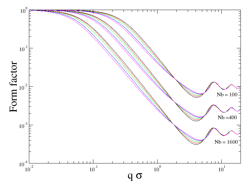
Form factor of KG polymers for changing stiffness. Shown are simulation data for the Kremer-Grest polymer melts for stiffness $\kappa$=0, 0.5, 1.0, 1.7, 2.15 (modelling cis-PI to PE, black to magenta colors) for block sizes $N_b=100,400,1600$ (the three bands of curves).

The figure above shows the polymer conformations as they would be measured in a neutron scattering study of a polymer melt. The melt consists of very long polymer chains, but they have been isotope labelled, such that we only observe the scattering from labelled sections containing $N_b$ beads and do not observe the scattering from all the non-labelled beads. Depending on size of the labelled sections we get the three bands of curves.

Within the three bands we show different polymer models with stiffnesses with different colours. KG models representing cis-PI are shown with black color (stiffness $\kappa=0$). KG models representing PE are shown with magenta color (stiffness $\kappa=2.15)$. These are the extremes in terms of stiffness, hence all other polymers would fall between these.

At low $q$ values / large scales the form factor contains information about the radius of gyration of the labelled sections of polymers. We observe that for increasing length of labels the corresponding radius of gyration also increases. Within each band, we also observe that for increasing chain stiffness the radius of gyration also increases. At intermediate $q$ values we observe the random walk chain statistics via the $q^{-2}$ power law which we expect from a polymer molecule. At even larger $q$ values and for stiff polymers such as PE, we see a cross-over to rod like scattering $q^{-1}$, whereas the random walk powerlaw persists for the flexible polymers such as cis-PI. At very $q~6\sigma$ values we see a peak and some oscillations. This is an artifact of the KG model where neighboring beads are separated by a bond length of about $1\sigma$ and this gives rise to a bragg peak, whereas for the real polymer we would have to do wide-angle scattering to see the carbon-carbon distance in the polymer backbone.

Exercise 2 changing stiffness (optional)

Inspired by the data above. We want to generate a several data sets of polymers with the same radius of gyration, but for varying stiffness. The radius of gyration is given by $R_g^2=b^2 N/6$. Note the result will not exactly look like the plot above, since we are changing both $N$ and $b$ simultaneously for the KG models.

• Choosing e.g. the PE polymer with $N=166$ steps and $b=15.40Å$ you used in exercise 1 as the polymer example. Generate the scattering for e.g. 0.25, 0.50, 0.75, 1.25, 1.50 times $b$. This corresponds to shorter/longer polymers with a different chemistry making them stiffer or more flexible. (Note the runtime of SEB depends on the number of units.)

Home

All SEB tutorials