Home

Tutorial: Lamellar Structures

Tutorial contributors: Andreas Haahr Larsen, Jacob Judas Kain Kirkensgaard.

Multilamellar lipid vesicle. Adapted from Luchini and Vitiello, 2021, Biomimetics 6: 3, with permission.

Before you start

Download and install SasView.

Learning outcomes

Understand the effect of form factors and structure factors on lamellar structures. You will be able to:

Understand how the scattering from lamellar structures looks (unilamellar vesicles, multilamellar vesicles).
Recognize scattering patterns with Bragg peaks from multilamellar structures.
Calculate SLDs and fit SAXS data of unilamellar and multilamellar structures using SasView.

Part I: Visual inspection of data

You have measured two SAXS datasets:

Sample1_clean.dat: DPPC in H₂O
Sample2_clean.dat: lecithin extract of unknown composition, but expected to contain much DPPC, also in H₂O.

The scientific question is: what structure do the different lipids form? The samples are either unilamellar or multilamellar vesicles:

Figure from Luchini and Vitiallo 2021 (reprinted with permission).
To visually assess the data, load the data into SasView and create a new plot (or other programs, e.g. PRIMUS or BioXTAS RAW, or plot the data manually, e.g. with python or MATLAB):

Observations:

Sample1.dat contains Bragg peaks, with the first order and second order peak being resolved. This is a sign of multilamellar structures, with the peaks stemming from the (center-to-center) distance between layers. Derive the layer distance from the positiona ($q$-values) of the Bragg peaks? (hint).
Sample2.dat does not have Bragg peaks, but is characteristic for the form factor of an unilammellar vesicle.
None of the datasets contain a Guinier region (see tutorial Primary Data Analysis), as the overall size of the vesicles are too large to be resolved in the measured $q$-range.

Part II: Pair distance distribution

A measured SAXS signal is a Fourier transformation of the sample. Therefore, one can try to Fourier tranform the data back, to get structural information, without having to do any fitting (for more information, see the tutorial Pair distance distribution).
Go to: BayesApp, which is a web application for doing indirect Fourier transformation of small-angle scattering data. Upload the Sample2.dat datafile to BayesApp, choose Transformation: Negative to allow for negative values of the pair distance distribution. Give an estimate for the maximum distance, e.g. 500 Å, set qmax to 0.5 Å^-1, and press Submit

The $p(r)$ display negative and positive parts. This is a sign of oscillations in electron density of the sample. That stems from the low density (relative to water) of the lipid tail groups and the high density (again, relative to water) of the lipid head groups. The first part of the $p(r)$, from 0 to ca 50 Å, corresponds to a bilayer, and the larger distances corresponds to the rest of the vesicle.
For Sample1.dat, you need to increase the number of points in $p(r)$ from the default 70 to, e.g., 200 (under Advanced options), to resolve the structural features. This makes BayesApp slower, but is necessary when $d_\mathrm{max}$ (the maximal distance in the sample) is large. Also, provide a larger estimate of the maximum distance, e.g. 800 Å. Press Submit

For Sample1.dat you will get a lot of oscillations in the $p(r)$. This corresponds to the many layers with positive and negative SLDs (positive: higher electron density than water, negative: lower electron density than water).

Part III: Fit the data with an analytical model

Before we fit the data, we need to consider all prior knowledge. This is critical because fitting SAS data is an ambiguous inverse problem, i.e. there are several models that can fit the data. First and foremost, we must estimate the scattering length densities (SLD) and excess scattering length density (ΔSLD = SLD - SLD_H2O) of DPPC head and tail groups. The molecular volumes can be determined experimentally and are 30 Å³ for H₂O, 325 Å³ for DPPC head groups (PC) and 969 Å³ for DPPC tail groups (DP). Use SasView's Density/Volume calculator (Tool -> Density/Volume calculator) to get the mass densities. You need to type in the chemical formula and molar volume. Be aware of unit conversion (hint).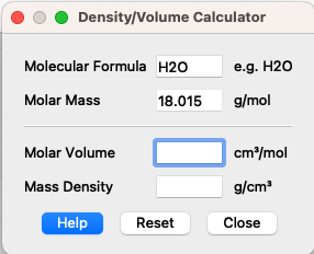

Then use SasView's SLD calculator to get the SLD values for solvent, head and tail group (solution).
Use the SasView models lamellar_hg (unilamellar vesicles) or lamellar_hg_stack_caille (multilamellar vesiceles) to fit the data. Start with Sample2.dat, as this data has the least features and therefore, most likely can be fitted easier.
When fitting a model to SAXS data, you would often not fit all parameters at once, you may follow this "protocol":

Protocol for fitting - simpler case of unilamellar vesicles

Select the dataset, press "Send data to" and select "Fitting" in the menu. Choose one of the models (under the category: Lamellae). Always start with the simplest model (in this case, that is lamellar_hg, unilamellar vesicles). You can add complexity if the simpler model does not fit data.
Before you fit the data, type in reasonable values for all parameters. DPPC has a tail length of 10-15 Å and a head length of 2-5 Å.
Calculate the scattering from the model (no fitting yet) by pressing "Compute/Plot".
Ignore the first point, by setting $q_\mathrm{min}=0.01$ (under Fit Options). Ignore the last points by setting $q_\mathrm{max}=0.5$
Fit scale and backbround (set a check-mark there and press "Fit"). Keep the other parameters fixed.
You may try to vary the parameters one at a time and press "Compute/Plot" to investigate what effect it has on the calculated scattering.
Now, try to fit length_tail and length_head (together with scale and background). This should give a reasonable fit. You may have to fix length_tail or set an upper limit, as a good fit can also be achieved for Sample2 with length_tail of around 15, which is unrealistic.
In the end, you may try to refine the scattering length densities, that you calculated. They should not be too different from the calculated values.
Correlation: you fit all SLDs (also solvent SLD), then you get "nan" as error-estimate on that parameter - why? (hint, or see the Spheres tutorial, Part I about correlated paramters).

For the model lamellar_hg_stack_caille (multilamellar vesiceles), there are some additional steps in the fitting protocol:

Protocol for fitting - more complex case of multilamellar vesicles

Before fitting, estimate a good initial value for the distance between layers, d_spacing, (see Part 1) and for the number of layers , Nlayers (see Part 2).
Ignore the first data point by setting $q_\mathrm{min}=0.01$ (under Fit Options). Ignore the last points by setting $q_\mathrm{max}=0.5$
Try to refine d_spacing by fitting this parameter together with scale, background and Caille_parameter.
(OBS: the model lamellar_hg_stack_caille has a bug, so Nlayers cannot be fitted - try to vary it manually instead.)
Then fit the length_tail and length_head. Are the values reasonable? else, try to fix one or set min/max values.
In the end, refine the scattering length densities. They should not be too different from the calculated values.

You will not get perfect fits (reduced $\chi^2$ are not unity) - this is ok. The fit may look like this for Sample2 (unilamellar) and like this for Sample1 (multilamellar). The goal was not to obtain perfect fits, but to answer the scientific question: what phase does the two lipid mixtures form?, and the models are sufficently good to answer that question. Other questions may also be answered with these models, e.g., how does the structure change if we change temperature, lipid composition, concenttration, etc
However, you may also consider how the models could be improved to get a more accurate fit (ideas).

Challenges

You have measured samples of phosholipids DMPC dissolved in H2O with SAXS, under two condition: after extrusion through at 50 nm filter (SAXS data DMPC 50 nm), or after extrusion with a 200 nm filter (SAXS data DMPC 200 nm). Describe the self-assembled structures of these samples. Regarding molecular volumes: DMPC has the same head group (PC) as DPPC (see Part III), but the tail group (DM) is different and has a molecular volume of 791 Å³.