Home

Tutorial: particle shapes and SAS patterns

Contributors: Andreas Haahr Larsen, Martin Cramer Pedersen.

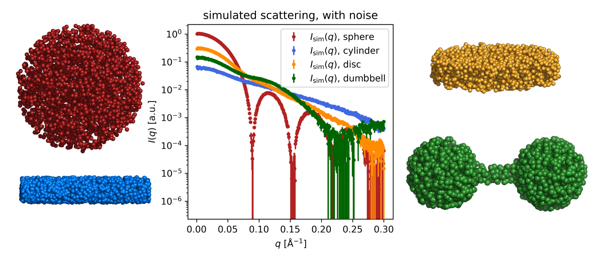
The scattering from various shapes (sphere, cylinder, disc and dumbbell) - simulated with Shape2SAS.

Before you start

No installation or prior knowledge is required for this tutorial.

Learning outcomes

Learn how various shapes translate into SAS patterns.

Simulate SAS data of different shapes.
Learn how particle size affects the scattering.
Recognize shapes (e.g., spheres, cylinders, and discs) directly from SAXS data.

Part I: Varying the size and its effect on the SAS data

Go to Shape2SAS, which can generate shapes and calculate the small-angle scattering from these shapes. Calculate the scattering from spheres of different sizes.

If the Shape2SAS webpage is empty, click the three lines in the upper-left corner and press Calculations.
Click the boxes Calculate scattering for Model 2/3/4.
Select the subunit type (in this case use the default: spheres). Only use 1 subunit in each model for this exercise.
The parameters a,b,c are the particle dimensions, but for spheres, you only need to change a, which is the radius. Choose different radii for each of the four spheres.
Press "Submit" to see the scattering (and 3D illustrations and 2D projections) of each sphere.
The scattering can optionally be plotted on a log-lin scale instead of a log-log scale (under Plotting options).
Notice the inverse effect of particle size: larger radius shift the minima to smaller values of $q$, and vice versa.

Assuming you want to measure these particles, and would like to capture both the first flat part (which is denoted the Guinier region as described in the Primary Data Analysis Tutorial) and the first few minima; What is the optimal $q$ range for measuring the simulated spheres with different sizes (if you will test, you can change the q_min and q_max in the top boxes of Shape2SAS)?
Changing the range of $q$ can be obtained by changing the instrument settings, i.e., changing sample-detector distance and/or wavelength.

Part II: Different shapes and their scattering patterns

Go to Shape2SAS, and try to generate the tutorial figure.

Select the subunit type. The dumbbell is generated by combining 3 subunits: 2 spheres and 1 cylinder, whereas the sphere, cylinder and disc consist of a single subunit.
The parameters a,b,c are the particle dimensions, and the meaning depends on the subunit type - hover the mouse over the boxes to get explanations.
The parameters x_com,y_com,z_com translates the center-off-mass of a given subunit.
Press "Submit" to see the scattering (and 3D illustrations) of each model.
The scattering can optionally be plotted on a log-lin scale instead of a log-log scale (Plotting options). This was done in the figure above.

Part III: Ambiguity. Different shapes, but similar SAS patterns.

Some shapes can result in rather similar SAS patterns. Go to Shape2SAS, and simulate 2 objects

Model: cylinder with radius 1 Å (a=b=10) and length 100 Å (c=100).
Model: an ellipsoid with axes 10, 10 and 70 (a=b=10 and c=70).

You may also compare a 50-Å sphere (a=50) with a 50-Å hollow sphere, with inner radius 20 Å (a=50,b=20).
Therefore, visual inspection of data, and pattern recognition is only the first step in analysis of SAXS or SANS data. Usually, more models are tested against the data, and any prior knowledge about the data (e.g. from microscopy or knowledge from the manufacturer) is considered in the analysis.

Challenges

Have a look at these SAXS data. What shapes could have been measured in each experiment, as assessed by the shape of the data? What shapes can be excluded with certainty?

Feedback

Help us improve the tutorials by

Reporting issues and bugs via our GitHub page. This could be typos, dead links etc., but also insufficient information or unclear instructions.
Suggesting new tutorials/additions/improvements in the SAStutorials forum.
Posting or answering questions in the SAStutorials forum.